LAB 2. Distribution layers

LAB 2. Distribution layers#

In this laboratory, We’ll understand how the tensorflow_probability.layers module works.

import inspect
from rlxmoocapi import submit, session

import numpy as np
import matplotlib.pyplot as plt
import seaborn as sns
import tensorflow as tf
import tensorflow_probability as tfp

from scipy import stats
from tensorflow.keras.layers import Dense, Input
from tensorflow.keras.optimizers import SGD
from tensorflow.keras.models import Model

tfd = tfp.distributions
tfpl = tfp.layers

course_id = "ppdl.v1"
endpoint = "https://m5knaekxo6.execute-api.us-west-2.amazonaws.com/dev-v0001/rlxmooc"
lab = "L02.03.02"

session.LoginSequence(
    endpoint=endpoint,
    course_id=course_id,
    lab_id=lab,
    varname="student"
    );

For this laboratory, We’ll learn the distribution parameters for each point in the following dataset:

x = np.linspace(0, 10, 100)
y = (
        .3 * x +
        2 * np.sin(x / 1.5) +
        np.random.normal(
            loc=.2,
            scale=.02 * ((x - 5) * 2) ** 2,
            size=(100, )
            )
        )

fig, ax = plt.subplots(1, 1, figsize=(10, 7))
ax.scatter(x, y)
ax.set_xlabel("$x$")
ax.set_ylabel("$y$")

Task 1#

In this task you must a feedforward neural network using using tensorflow.keras.models.Model. This model must output an independent normal distribution.

NOTE: the dense layer that represents the distribution parameters must have a linear activation.

def make_model(hidden_units, activation, input_shape):
    # YOUR CODE HERE
    return Model()

The summary of your model must be equivalent to this one:

model_summary

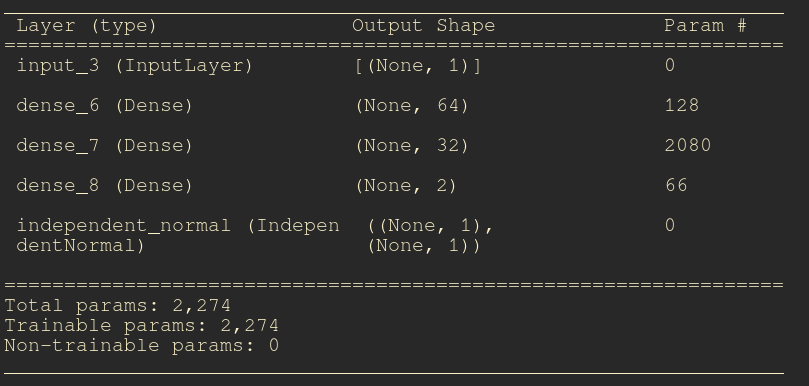
model = make_model(
        hidden_units=[64, 32],
        activation="relu",
        input_shape=1,
        event_shape=1
        )
model.summary()

Test your code:

student.submit_task(namespace=globals(), task_id="T1");

model.summary()

We can visualize the density of the model (untrained):

dist = model(x.reshape(-1, 1))
means = dist.mean().numpy().flatten()
stds = dist.stddev().numpy().flatten()

fig, ax = plt.subplots(figsize=(7, 7))
ax.plot(x, means) 
ax.fill_between(x, means - 3 * stds, means + 3 * stds, alpha=0.5)

Task 2#

Implement the train_model function, which must compute the loss for a maximum likelihood estimation problem:

\[\begin{split} \mathcal{L} = -\frac{1}{N}\text{log}(P_x(y))\\ P_x(y) = \mathcal{N}(\mu=f_1(x), \sigma=f_2(x)) \end{split}\]

Where \(f_1(\cdot)\) and \(f_2(\cdot)\) are functions approximated through the feedforward neural network.

def train_model(model, x, y, epochs, optimizer):
    ## YOUR CODE HERE
    for epoch in range(epochs):
        with tf.GradientTape() as t:
            loss = ...
        grads = t.gradient(..., ...)
        optimizer.apply_gradients(zip(..., ...))
        print(f"epoch: {epoch}, loss: {float(loss.numpy())}")

train_model(model, x, y, 2000, SGD(learning_rate=0.01))

student.submit_task(namespace=globals(), task_id="T2");

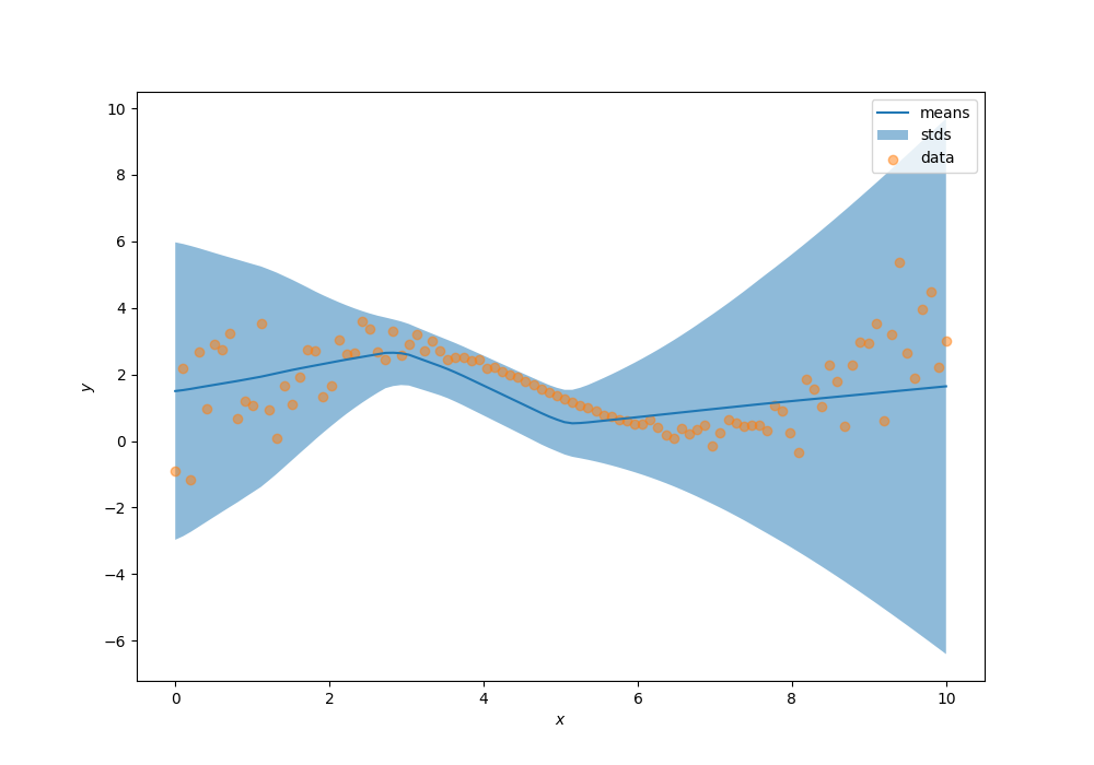
Now, let’s visualize the learned distributions, your predictions must look similar to the following result:

regression_dist

dist = model(x.reshape(-1, 1))
means = dist.mean().numpy().flatten()
stds = dist.stddev().numpy().flatten()

fig, ax = plt.subplots(1, 1, figsize=(10, 7))
ax.plot(x, means, label="means") 
ax.fill_between(x, means - 3 * stds, means + 3 * stds, alpha=0.5, label="stds")
ax.scatter(x, y, alpha=0.5, label="data")
ax.legend()
ax.set_xlabel("$x$")
ax.set_ylabel("$y$")

Task 3#

Implement the log_prob function without tensorflow_probability or tensorflow. You can use numpy and scipy.stats. This function receives as arguments the data (x, y), and the neural network parameters weights.

NOTE 1: you must transform the rstd (\(\hat{\sigma}\)) into valid standard deviations, with a softplus transformation:

\[ \sigma = \text{log}(\text{exp}(\hat{\sigma}) + 1) \]

NOTE 2: your function must support models with different layers sizes, you can test your function creating models with different number of layers and units.

weights = [layer.get_weights() for layer in model.layers[1:-1]]

print(len(weights))

# parameters for layer 1
w, b = weights[0]
print(w)
print(b)

pdf1 = pdf(x, y, weights)
pdf1[:10]

dist = model(x.reshape(-1, 1))
pdf2 = np.exp(dist.log_prob(y.reshape(-1, 1)))
pdf2[:10]

You can visualize that both log probs are the same:

data1 = np.array(sorted(zip(y, pdf1), key=lambda x: x[0])).T
data2 = np.array(sorted(zip(y, pdf2), key=lambda x: x[0])).T

fig, ax = plt.subplots(1, 2, figsize=(10, 7))
ax[0].plot(data1[0], data1[1])
ax[0].fill_between(
        data1[0], np.zeros((100, )), data1[1], alpha=0.4
        )
ax[0].set_title("Your solution")

ax[1].plot(data2[0], data2[1])
ax[1].fill_between(
        data2[0], np.zeros((100, )), data2[1], alpha=0.4
        )
ax[1].set_title("Tensorflow probability")

student.submit_task(namespace=globals(), task_id="T3");

Task 4#

Compute the gradients for the probabilistic layer in the model without tensorflow. You can use numpy and scipy.

Consider the loss function:

\[\begin{split} \mathcal{L}(\mu_i, \sigma_i) = \text{log}(\mathcal{N}(\mu_i, \sigma_i))\\ \frac{\partial \mathcal{L}(\mu_i, \sigma_i)}{\partial \mu_i} = ?\\ \end{split}\]

NOTE: you must transform the rstd (\(\hat{\sigma}\)) into valid standard deviations, with a softplus transformation: